Vectors in theory
Contents
1. Vectors in theory
I want to point out that the class of abstract linear spaces is no larger than the class of spaces whose elements are arrays. So what is gained by abstraction? First of all, the freedom to use a single symbol for an array; this way we can think of vectors as basic building blocks, unencumbered by components. The abstract view leads to simple, transparent proofs of results. — Peter D. Lax, in Chapter 1 of his book Linear Algebra and its Applications
The mathematics of machine learning rest upon three pillars: linear algebra, mathematical analysis, and probability theory. Linear algebra describes how to represent and manipulate data; mathematical analysis helps us define and fit models; while probability theory helps interpret them.
These are building on top of each other, and we will start at the beginning: representing and manipulating data.
1.1. Representing data
To guide us throughout this section, we will look at the famous Iris dataset. This contains the measurements from three species of Iris: the lengths and widths of sepals and petals. Each data point includes these four measurements, and we also know the corresponding species (Iris setosa, Iris virginica, Iris versicolor).
The dataset can be loaded right away from scikit-learn, so let’s take a look!
from sklearn.datasets import load_iris

data = load_iris()

X, y = data["data"], data["target"]
X[:10]
array([[5.1, 3.5, 1.4, 0.2],
       [4.9, 3. , 1.4, 0.2],
       [4.7, 3.2, 1.3, 0.2],
       [4.6, 3.1, 1.5, 0.2],
       [5. , 3.6, 1.4, 0.2],
       [5.4, 3.9, 1.7, 0.4],
       [4.6, 3.4, 1.4, 0.3],
       [5. , 3.4, 1.5, 0.2],
       [4.4, 2.9, 1.4, 0.2],
       [4.9, 3.1, 1.5, 0.1]])
Before going into the mathematical definitions, let’s establish a common vocabulary first. The measurements
themselves are stored in a tabular format. Rows represent samples, and columns represent measurements. A particular
measurement type is often called feature. As
X.shape tells us, the Iris dataset has
150 data points and four features.
X.shape
(150, 4)
For a given sample, the corresponding species is called the label. In our case, this is either Iris setosa, Iris virginica, or Iris versicolor. Here, the labels are encoded with the numbers 0, 1, and 2.
y
array([0, 0, 0, 0, 0, 0, 0, 0, 0, 0, 0, 0, 0, 0, 0, 0, 0, 0, 0, 0, 0, 0,
       0, 0, 0, 0, 0, 0, 0, 0, 0, 0, 0, 0, 0, 0, 0, 0, 0, 0, 0, 0, 0, 0,
       0, 0, 0, 0, 0, 0, 1, 1, 1, 1, 1, 1, 1, 1, 1, 1, 1, 1, 1, 1, 1, 1,
       1, 1, 1, 1, 1, 1, 1, 1, 1, 1, 1, 1, 1, 1, 1, 1, 1, 1, 1, 1, 1, 1,
       1, 1, 1, 1, 1, 1, 1, 1, 1, 1, 1, 1, 2, 2, 2, 2, 2, 2, 2, 2, 2, 2,
       2, 2, 2, 2, 2, 2, 2, 2, 2, 2, 2, 2, 2, 2, 2, 2, 2, 2, 2, 2, 2, 2,
       2, 2, 2, 2, 2, 2, 2, 2, 2, 2, 2, 2, 2, 2, 2, 2, 2, 2])
In its entirety, the Iris dataset forms a matrix, and the data points form vectors. Simply speaking, matrices are tables, while vectors are tuples of numbers. (Tuples are are just finite sequence of numbers, like \( (1.297, -2.35, 32.3, 29.874) \).) However, this view doesn’t give us the big picture. Moreover, since we have more than three features, we cannot visualize the dataset easily. As humans cannot see in more than three dimensions, visualization breaks down.
Besides representing the data points in a compact form, we want to perform operations on them, like addition and scalar multiplication. Why do we need to add data points together? To give you a simple example, it is often beneficial if the features are on the same scale. If a given feature is distributed on a smaller scale than the others, it will have less influence on the predictions.
Think about this: if somebody is whispering to you something from the next room while speakers blast loud music right next to your ear, you won’t hear anything from what the person is saying to you. Large-scale features are the blasting music, while the smaller ones are the whisper. You may obtain much more information from the whisper, but you need to quiet down the music first.
To see this phenomenon in action, let’s take a look at the distribution of the features of our dataset!
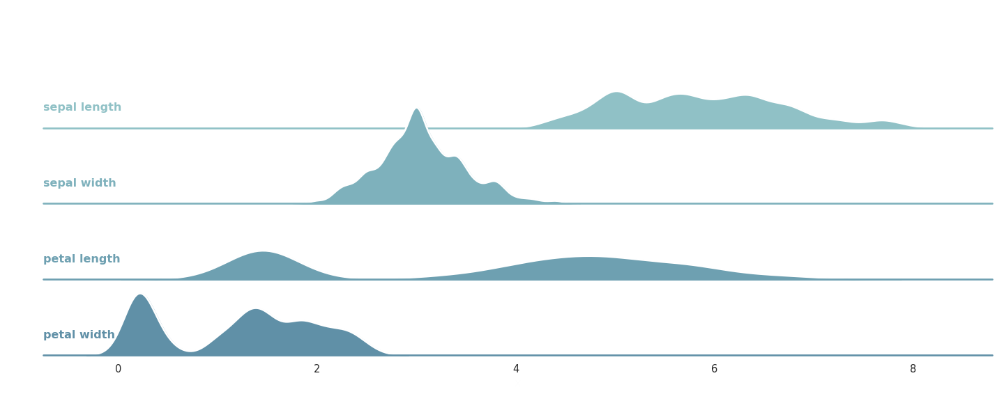
Fig. 1.1 Distribution of the individual features of the Iris dataset.
You can see in Fig. 1.1 that some are more stretched-out (like the sepal length), while others are narrower (like sepal width). In practical scenarios, this can hurt the predictive performance of our algorithms.
To solve it, we can remove the mean and the standard deviation of a dataset. If the dataset consists of the vectors \( x_1, x_2, \dots, x_{150} \), we can calculate their mean by
and their standard deviation by
where the square operation in \( (x_i - \mu)^2 \) is taken elementwise. The components of \( \mu = (\mu_1, \mu_2, \mu_3, \mu_4) \) and \( \sigma = (\sigma_1, \sigma_2, \sigma_3, \sigma_4) \) are the means and variances of the individual features. (Recall that the Iris dataset contains 150 samples and 4 features per sample.)
In other words, the mean describes the average of samples, while the standard deviation represents the average distance from the mean. The larger the standard deviation is, the more spread out the samples are.
With these quantities, the scaled dataset can be described as
where both the substraction and the division are taken elementwise.
If you are familiar with Python and NumPy, this is how it is done. (Don’t worry if you are not, everything you need to know about them will be explained in the next chapter, with example code.)
X_scaled = (X - X.mean(axis=0))/X.std(axis=0)
X_scaled[:10]
array([[-0.90068117,  1.01900435, -1.34022653, -1.3154443 ],
       [-1.14301691, -0.13197948, -1.34022653, -1.3154443 ],
       [-1.38535265,  0.32841405, -1.39706395, -1.3154443 ],
       [-1.50652052,  0.09821729, -1.2833891 , -1.3154443 ],
       [-1.02184904,  1.24920112, -1.34022653, -1.3154443 ],
       [-0.53717756,  1.93979142, -1.16971425, -1.05217993],
       [-1.50652052,  0.78880759, -1.34022653, -1.18381211],
       [-1.02184904,  0.78880759, -1.2833891 , -1.3154443 ],
       [-1.74885626, -0.36217625, -1.34022653, -1.3154443 ],
       [-1.14301691,  0.09821729, -1.2833891 , -1.44707648]])
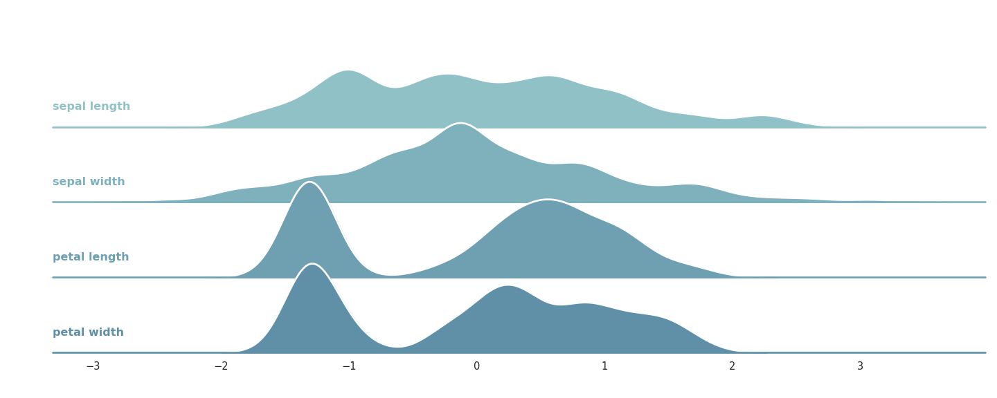
Fig. 1.2 Features of the Iris dataset after scaling.
If you compare this modified version with the original, you can see that its features are on the same scale. From a (very) abstract point of view, machine learning is nothing else but a series of learned data transformations, turning raw data into a form where prediction is simple.
In a mathematical setting, manipulating data and modeling its relations to the labels arise from the concept of vector spaces and transformations between them. Let’s take the first steps by making the definition of vector spaces precise!
1.2. What is a vector space?
Representing multiple measurements as a tuple \( (x_1, x_2, \dots, x_n) \) is a natural idea that has a ton of merits. The tuple form suggests that the components belong together, giving a clear and concise way to store information.
However, this comes at a cost: now we have to deal with more complex objects. Despite having to deal with objects like \( (x_1, \dots, x_n) \) instead of numbers, there are similarities. For instance, if \( x = (x_1, \dots, x_n) \) and \( y = (y_1, \dots, y_n) \) are two arbitrary tuples,
-
they can be added together by \( x + y = (x_1 + y_1, \dots, x_n + y_n) \),
-
and they can be multiplied with scalars: if \( c \in \mathbb{R} \), then \( c x = (c x_1, \dots, c x_n) \).
It’s almost like using a number.
These operations have clear geometric interpretations as well. Adding two vectors together is the same as translation, while multiplying with a scalar is a simple stretching. (Or squeezing, if \( |c| < 1 \).)
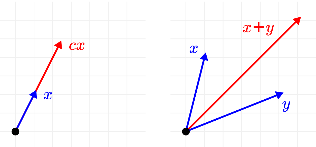
Fig. 1.3 Geometric interpretation of addition and scalar multiplication.
On the other hand, if we want to follow our geometric intuition (which we definitely do), it is unclear how to define vector multiplication. The definition
might make sense algebraically, but it is unclear what it means in a geometric sense.
When we think about vectors and vector spaces, we are thinking about a mathematical structure that fits our intuitive views and expectations. So, let’s turn these into the definition!
Definition 1.1 (Vector spaces.)
A vector space is a mathematical structure \( (V, F, +, \cdot) \), where
(a) \( V \) is the set of vectors,
(b) \( + : V \times V \to V \) is the addition operation, satisfying
-
\( x + y = y + x \) (commutativity),
-
\( x + (y + z) = (x + y) + z \) (associativity),
-
there is an element \( 0 \in V \) such that \( x + 0 = x \) (existence of the null vector),
-
there is an inverse \( -x \in V \) for each \( x \in V \) such that \( x + (-x) = 0 \) (existence of additive inverses)
for all vectors \( x, y, z \in V \),
(c) \( F \) is a field of scalars (most commonly the real numbers \( \mathbb{R} \) or the complex numbers \( \mathbb{C} \)),
(d) and \( \cdot: F \times V \to V \) is the scalar multiplication operation, satisfying
-
\( a(bx) = (ab) x \) (associativity),
-
\( a(x + y) = ax + ay \) (distributivity),
-
\( 1x = x \)
for all scalars \( a, b \in F \) and vectors \( x, y \in V \).
This definition is overloaded with new concepts, so we need to unpack it.
First, looking at operations like addition and scalar multiplication as functions might be unusual for you, but this is a perfectly natural representation. In writing, we use the notation \( x + y \), but when thinking about \( + \) as a function of two variables, we might as well write \( +(x, y) \). The form \( x + y \) is called infix, while \( +(x, y) \) is called prefix notations.
In vector spaces, the input of addition are two vectors and the result is a single vector, thus \( + \) is a function that maps the Cartesian product \( V \times V \) to \( V \). Similarly, scalar multiplication takes a scalar and a vector, resulting in a vector; meaning a function that maps \( F \times V \) to \( V \).
This is also good place to note that mathematical definitions are always formalized in hindsight after the objects themselves are somewhat crystallized and familiar to the users. Mathematics is often presented as definitions first, then theorems second, but this is not how it is done in practice. Examples motivate definitions, not the other way around.
In general, the field of scalars can be something other than real or complex numbers. The term field refers to a well-defined mathematical structure, which turns a natural notion mathematically precise. Without going into the technical details, we will think about fields as “a set of numbers where addition and multiplication works just as for real numbers”.
Since we are not concerned with the most general case, we will use \( \mathbb{R} \) or \( \mathbb{C} \) to avoid unnecessary difficulty. If you are not familiar with the exact mathematical definition of a field, don’t worry, just think of \( \mathbb{R} \) each time you read the word “field”.
When everything is clear from the context, \( (V, \mathbb{R}, +, \cdot) \) will be often referred to as \( V \) for notational simplicity. So, if the field \( F \) is not specified, it is implicitly assumed to be \( \mathbb{R} \). When we want to emphasize this, we’ll call these real vector spaces.
At first sight, this definition is certainly too complex to comprehend. It seems like just a bunch of sets, operations, and properties thrown together. However, to help us build a mental model, we can imagine a vector as an arrow, starting from the null vector. (Recall that the null vector \( 0 \) is that special one for which \( x + 0 = x \) holds for all \( x \). Thus, it can be considered as an arrow with zero length; the origin.)
To further familiarize ourselves with the concept, let’s see some examples of vector spaces!
1.3. Examples of vector spaces
Examples are one of the best ways of building insight and understanding of seemingly difficult concepts like vector spaces. We, humans, usually think in terms of models instead of abstractions. (Yes, this includes pure mathematicians. Even though they might deny it.)
Example 1. The most ubiquitous instance of the vector space is \( (\mathbb{R}^n, \mathbb{R}, +, \cdot) \), the same one we used to motivate the definition itself. (\( \mathbb{R}^n \) refers to the n-fold Cartesian product of the set of real numbers. If you are unfamiliar with this notion, check the set theory tutorial in the Appendix.)
\( (\mathbb{R}^n, \mathbb{R}, +, \cdot) \) is the canonical model, the one we use to guide us throughout our studies. If \( n = 2 \), we are simply talking about the familiar Euclidean plane.
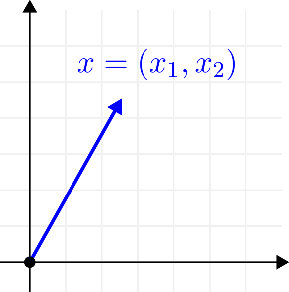
Fig. 1.4 The Euclidean plane as a vector space.
Using \( \mathbb{R}^2 \) or \( \mathbb{R}^3 \) for visualization can help a lot. What works here will usually work in the general case, although sometimes this can be dangerous. Math relies on both intuition and logic. We develop ideas using our intuition, but we confirm them with our logic.
Example 2. Not all vector spaces take the form of a collection of finite tuples. An example of this is the space of polynomials with real coefficients, defined by
Two polynomials \( p(x) \) and \( q(x) \) can be added together by
and can be multiplied with a real scalar by
With these operations, \( (\mathbb{R}[x], \mathbb{R}, +, \cdot) \) is a vector space. Although most of the time we percieve polynomials as functions, they can be represented as tuples of coefficients as well:
Note that \( n \), the degree of the polynomial, is unbounded. As a consequence, this vector space has a significantly richer structure than \( \mathbb{R}^n \).
Example 3. The previous example can be further generalized. Let \( C([0, 1]) \) denote the set of all continuous real functions \( f: [0, 1] \to \mathbb{R} \). Then \( (C(\mathbb{R}), \mathbb{R}, +, \cdot) \) is a vector space, where the addition and scalar multiplication are defined just as in the previous example:
for all \( f, g \in C(\mathbb{R}) \) and \( c \in \mathbb{R} \).
Yes, that is right: functions can be thought of as vectors as well. Spaces of functions play a significant role in mathematics, and they come in several different forms. We often restrict the space to continuous functions, differentiable functions, or basically any subset that is closed under the given operations.
(In fact, \( \mathbb{R}^n \) can be also thought of as a function space. From an abstract viewpoint, each vector \( x = (x_1, \dots, x_n) \) is a mapping from \( \{1, 2, \dots, n \} \) to \( \mathbb{R} \).)
Function spaces are encountered in more advanced topics, such as inverting ResNet architectures, which we won’t deal with in this book. However, it is worth seeing examples that are different (and not as straightforward) as \( \mathbb{R}^n \).
1.4. Linear basis
Although our vector spaces contain infinitely many vectors, we can reduce the complexity by finding special subsets that can express any other vector.
To make this idea precise, let’s consider our recurring example \( \mathbb{R}^n \). There, we have a special vector set
which can be used to express each element \( x = (x_1, \dots, x_n) \) as
For instance, \( e_1 = (1, 0) \) and \( e_2 = (0, 1) \) in \( \mathbb{R}^2 \).
What we have just seen feels extremely trivial and it seems to only complicate things. Why would we need to write vectors in the form of \( x = \sum_{i=1}^{n} x_i e_i \), instead of simply using the coordinates \( (x_1, \dots, x_n) \)? Because, in fact, the coordinate notation depends on the underlying vector set (\( \{e_1, \dots, e_n\} \) in our case) used to express other vectors.
A vector is not the same as its coordinates! A single vector can have multiple different coordinates in different systems, and switching between these is a useful tool.
Thus, the set \( E = \{ e_1, \dots, e_n \} \subseteq \mathbb{R}^n \) is rather special, as it significantly reduces the complexity of representing vectors. With the vector addition and scalar multiplication operations, it spans our vector space entirely. \( E \) is an instance of a vector space basis, a set that serves as a skeleton of \( \mathbb{R}^n \).
In this section, we are going to introduce and study the concept of vector space basis in detail.
1.4.1. Linear combinations and independence
Let’s zoom out from the special case \( \mathbb{R}^n \) and start talking about general vector spaces. From our motivating example regarding bases, we have seen that sums of the form
where the \( v_i \)-s are vectors and the \( x_i \) coefficients are scalars, play a crucial role. These are called linear combinations. A linear combination is called trivial if all of the coefficients are zero.
Given a set of vectors, the same vector can potentially be expressed as a linear combination in multiple ways. For example, if \( v_1 = (1, 0), v_2 = (0, 1) \), and \( v_3 = (1, 1) \), then
This suggests that the set \( S = \{ v_1, v_2, v_3 \} \) is redundant, as it contains duplicate information. The concept of linear dependence and independence makes this precise.
Definition 1.2 (Linear dependence and independence.)
Let \( V \) be a vector space and \( S = \{ v_1, \dots, v_n \} \) be a subset of its vectors. \( S \) is said to be linearly dependent if it only contains the zero vector, or there is a nonzero \( v_k \) that can be expressed as a linear combination of the other vectors \( v_1, \dots, v_{k-1}, v_{k+1}, \dots, v_n \).
\( S \) is said to be linearly independent if it is not linearly dependent.
Linear dependence and independence can be looked at from a different angle. If
for some nonzero \( v_k \), then by subtracting \( v_k \), we obtain that the null vector can be obtained as a nontrivial linear combination
for some scalars \( x_i \), where \( x_k = -1 \). This is an equivalent definition of linear dependence. With this, we have proved the following theorem.
Theorem 1.1
Let \( V \) be a vector space and \( S = \{ v_1, \dots, v_n \} \) be a subset of its vectors.
(a) \( S \) is linearly dependent if and only if the null vector \( 0 \) can be obtained as a nontrivial linear combination.
(b) \( S \) is linearly independent if and only if whenever \( 0 = \sum_{i=1}^{n} x_i v_i \), all coefficients \( x_i \) are zero.
1.4.2. Spans of vector sets
Linear combinations provide a way to take a small set of vectors and generate a whole lot of others from them. For a set of vectors \( S \), taking all of its possible linear combinations is called spanning, and the generated set is called the span. Formally, it is defined by
Note that the vector set \( S \) is not necessarily finite. To help illustrate the concept of span, we can visualize the process in three dimensions. The span of two linearly independent vectors is a plane.
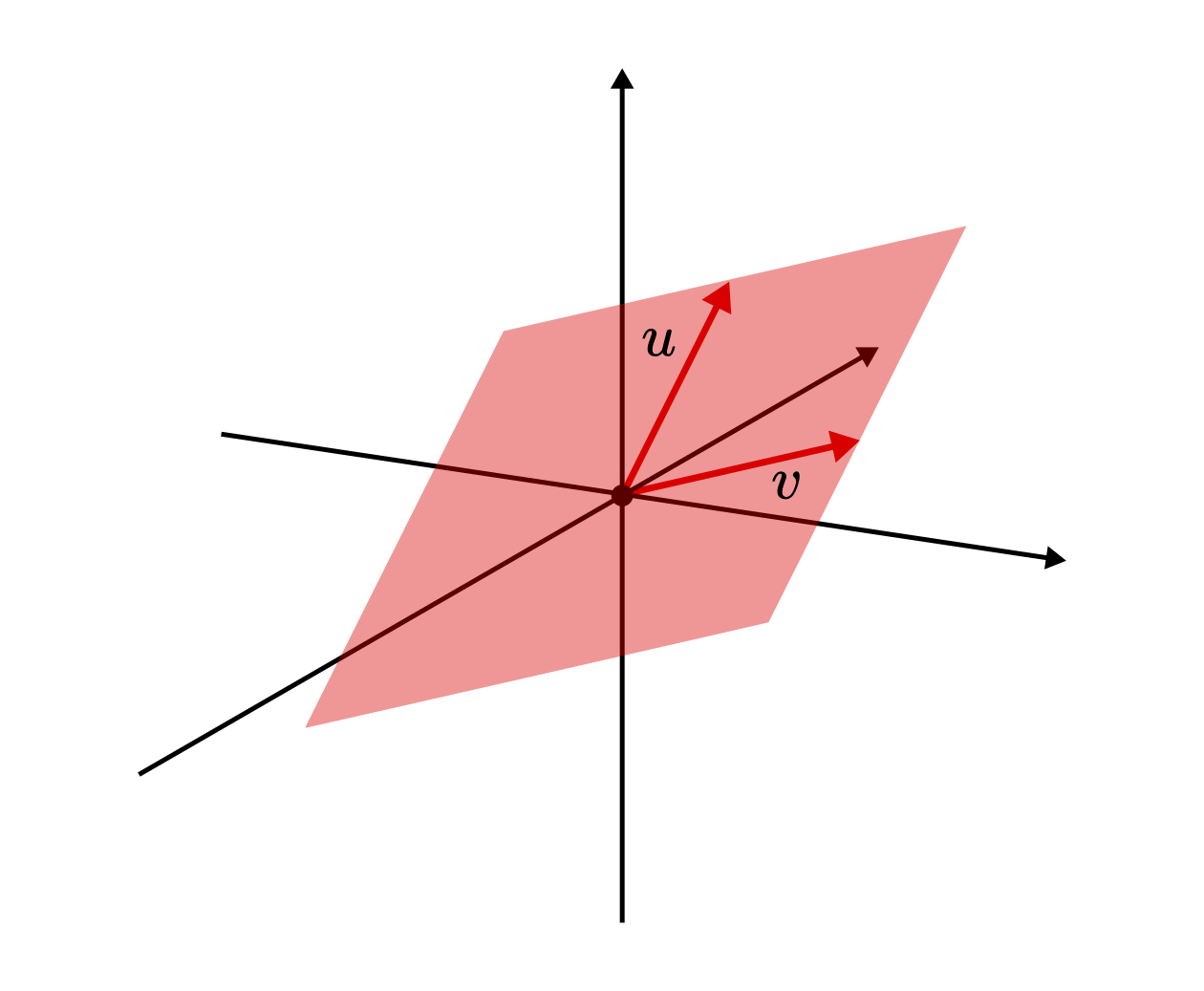
Fig. 1.5 The span of two linearly independent vectors \( u \) and \( v \) in \( \mathbb{R}^3 \).
Sometimes, when we are talking about spans of a finite vector set \( \{v_1, \dots, v_n \} \), we denote the span as
This can help us to avoid overcomplicating notations by naming every set.
There are some obvious properties of the span, for instance, if \( S_1 \subseteq S_2 \), then \( \mathrm{span}(S_1) \subset \mathrm{span}(S_2) \). Moreover, the span is closed under linear combinations, so \( \mathrm{span}(\mathrm{span}(S)) = \mathrm{span}(S) \). Because of this, if \( S \) is linearly dependent, we can remove the redundant vectors and still keep the span the same.
Think about it: if \( S = \{ v_1, \dots, v_n \} \) and, say, \( v_n = \sum_{i=1}^{n-1} x_i v_i \), then \( v_n \in \mathrm{span}(S \setminus \{v_n\}) \). So,
Among sets of vectors, those that generate the entire vector space are special. Remember that we started the discussion about linear combinations to find subsets that can be used to express any vector. After all this setup, we are ready to make a formal introduction. Any set of vectors \( S \) that have the property \( \mathrm{span}(S) = V \) is called a generating set for \( V \).
\( S \) can be thought of as a “lossless compression” of \( V \), as it contains all the information needed to reconstruct any element in \( V \), yet it is smaller than the entire space. Thus, it is natural to aim to reduce the size of the generating set as much as possible. This leads us to one of the most important concepts in linear algebra: minimal generating sets, or bases, as we prefer to call them.
1.4.3. Bases, the minimal generating sets
With all the intuition we have built so far, let’s jump into the definition right away!
Definition 1.3 (Basis.)
Let \( V \) be a vector space and \( S \) be a subset of its vectors. \( S \) is a basis of \( V \) if
(a) \( S \) is linearly independent,
(b) and \( \mathrm{span}(S) = V \).
The elements of a basis set are called basis vectors.
It can be shown that these defining properties mean that every vector \( x \) can be uniquely written as a linear combination of \( S \). (This is left as an exercise for the reader)
Let’s see some examples! In \( \mathbb{R}^3 \), the set \( \{ (1, 0, 0), (0, 1, 0), (0, 0, 1) \} \) is a basis, but so is \( \{ (1, 1, 1), (1, 1, 0), (0, 1, 1) \} \). So, there can be more than one basis for the same vector space.
For \( \mathbb{R}^n \), the most commonly used basis is \( \{ e_1, \dots, e_n \} \), where \( e_i \) is a vector whose all coordinates are 0, except the \( i \)-th one, which is \( 1 \). This is called the standard basis.
In terms of the “information” contained in a set of vectors, bases hit the sweet spot. Adding any new vector to a basis set would introduce redundancy; removing any of its elements would cause the set to be incomplete. These notions are formalized in the two theorems below.
Theorem 1.2
Let \( V \) be a vector space and \( S = \{ v_1, \dots, v_n \} \) a subset of vectors. The following are equivalent.
(a) \( S \) is a basis.
(b) \( S \) is linearly independent and for any \( x \in V \setminus S \), the vector set \( S \cup \{ x \} \) is linearly dependent. In other words, \( S \) is a maximal linearly independent set.
Proof. To show the equivalence of two propositions, we have to prove two things: that (a) implies (b); and that (b) implies (a). Let’s start with the first one!
(a) \( \implies \) (b) If \( S \) is a basis, then any \( x \in V \) can be written as \( x = \sum_{i=1}^{n} x_i v_i \) for some \( x_i \in \mathbb{R} \). Thus, by definition, \( E \cup \{ x \} \) is linearly dependent.
(b) \( \implies \) (a). Our goal is to show that any \( x \) can be written as a linear combination of the vectors in \( S \). By our assumption, \( S \cup \{ x \} \) is linearly dependent, so \( 0 \) can be written as a nontrivial linear combination:
where not all coefficients are zero. Because \( S \) is linearly independent, \( \alpha \) cannot be zero. (As it would imply the linear dependence of \( S \), which would go against our assumptions.) Thus,
showing that \( S \) is a basis. \( \square \)
Next, we are going to show that every vector of a basis is essential.
Theorem 1.3
Let \( V \) be a vector space and \( S = \{ v_1, \dots, v_n \} \) a basis. Then for any \( v \in S \), the span of \( S \setminus \{ v \} \) is a proper subset of \( V \).
Proof. We are going to prove by contradiction. Without the loss of generality, we can assume that \( v = v_1 \). If \( \mathrm{span}(S \setminus \{v_1\}) = V \), then
This means that \( S = \{ v_1, \dots, v_n \} \) is not linearly independent, contradicting our assumptions. \( \square \)
In other words, the above results mean that a basis is a maximal linearly independent and a minimal generating set at the same time.
Given a basis \( S = \{ v_1, \dots, v_n \} \), we implictly write the vector \( x = \sum_{i=1}^{n} x_i v_i \) as \( x = (x_1, \dots, x_n) \). Since this decomposition is unique, we can do this without issues. The coefficients \( x_i \) are also called coordinates. (Note that the coordinates strongly depend on the basis. Given two different bases, the coordinates of the same vector can be different.)
1.4.4. Finite dimensional vector spaces
As we have seen previously, bases are not unique, as a single vector space can have many different bases. A very natural question that arises in this context is the following. If \( S_1 \) and \( S_2 \) are two bases for \( V \), then does \( |S_1| = |S_2| \) hold? (Where \( |S| \) denotes the cardinality of the set \( S \), that is, its “size”.)
In other words, can we do better if we select our basis more cleverly? It turns out that we cannot, and the sizes of any two basis sets is equal. We are not going to prove this, but here is the theorem in its entirety.
Theorem 1.4
Let \( V \) be a vector space and \( S_1 \), \( S_2 \) be two of its bases. Then \( |S_1| = |S_2| \).
This gives us a way to define the dimension of a vector space, which is simply the cardinality of its basis. We’ll denote the dimension of \( V \) as \( \dim(V) \). For example, \( \mathbb{R}^n \) is \( n \)-dimensional, as shown by the standard basis \( \{ (1, 0, \dots, 0), \dots, (0, 0, \dots, 1) \} \).
If you recall the previous theorems, we almost always assumed that a basis is finite. You might ask the question: is this always true? The answer is no. Examples 2 and 3 show that this is not the case. For instance, the countably infinite set \( \{ 1, x, x^2, x^3, \dots \} \) is a basis for \( \mathbb{R}[x] \). So, according to the theorem above, no finite basis can exist there.
This marks an important distinction between vector spaces: those with finite bases are called finite-dimensional. I have some good news: all finite-dimensional real vector spaces are essentially \( \mathbb{R}^n \). (Recall that we call a vector space real if its scalars are the real numbers.)
To see why, suppose that \( V \) is an \( n \)-dimensional real vector space with basis \( \{ v_1, \dots, v_n \} \), and define the mapping \( \varphi: V \to \mathbb{R}^n \) by
\( \varphi \) is invertible and preserves the structure of \( V \), that is, the addition and scalar multiplication operations. Indeed, if \( u, v \in V \) and \( \alpha, \beta \in \mathbb{R} \), then \( \varphi(\alpha u + \beta v) = \alpha \varphi(x) + \beta \varphi(y) \). Such mappings are called isomorphisms. The word itself is derived from ancient Greek, with isos meaning same and morphe meaning shape. Even though this sounds abstract, the existence of an isomorphism between two vector spaces mean that they have the same structure. So, \( \mathbb{R}^n \) is not just an example of finite dimensional real vector spaces, it is a universal model of them. (Note that if the scalars are not the real numbers, the isomorphism to \( \mathbb{R}^n \) is not true.)
Considering that we’ll almost exclusively deal with finite dimensional real vector spaces, this is good news. Using \( \mathbb{R}^n \) is not just a heuristic, it is a good mental model.
1.4.5. Why are bases so important?
If every finite-dimensional real vector space is essentially the same as \( \mathbb{R}^n \), what do we gain from abstraction? Sure, we can just work with \( \mathbb{R}^n \) without talking about bases, but to develop a deep understanding of the core mathematical concepts in machine learning, we need the abstraction.
Let’s look ahead briefly and see an example. If you have some experience with neural networks, you know that matrices play an essential role in defining its layers. Without any context, matrices are just a table of numbers with seemingly arbitrary rules of computation. Have you ever wondered why matrix multiplication is defined the way it is?
Although we haven’t precisely defined matrices yet, you have probably encountered them previously. For two matrices
their product is defined by
that is, the \( i, j \)-th element of \( AB \) is defined by
Even though we can visualize this to make it easier to understand, the definition seems random.
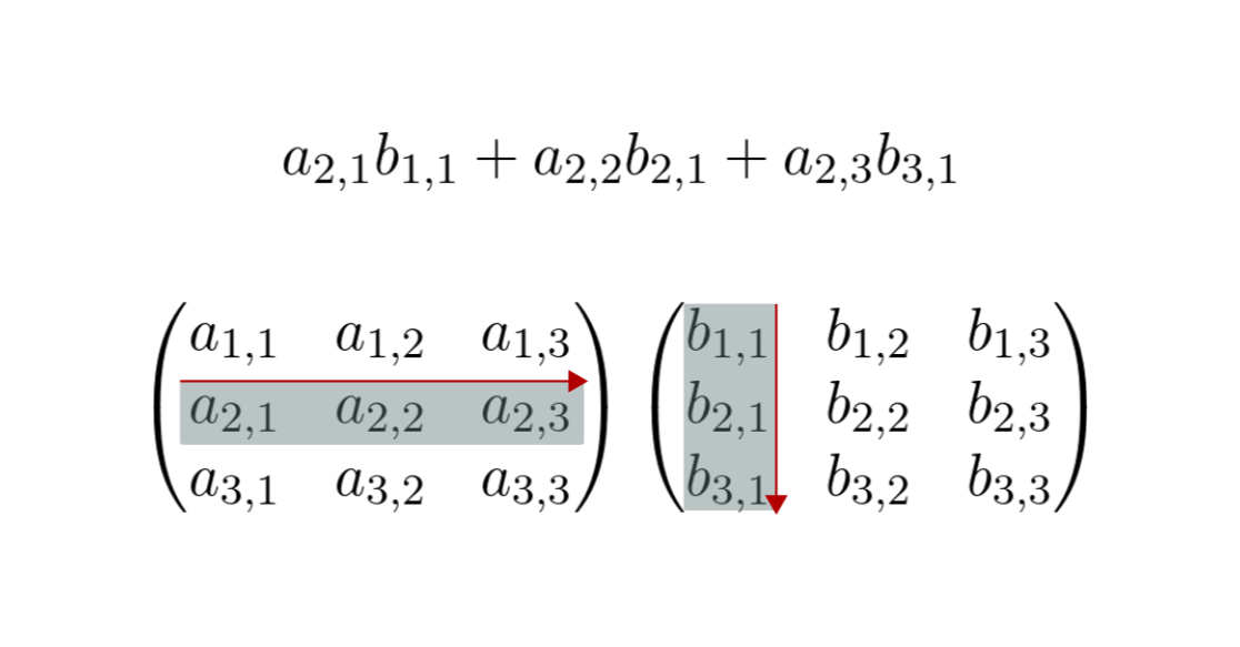
Fig. 1.6 Matrix multiplication visualized.
Why not just take the componentwise product \( (a_{i,j} b_{i,j})_{i,j=1}^{n} \)? The definition becomes crystal clear once we look at a matrix as a tool to describe linear transformations between vector spaces, as the elements of the matrix describe the images of basis vectors. In this context, multiplication of matrices is just the composition of linear transformations.
Instead of just putting out the definition and telling you how to use it, I want you to understand why it is defined that way. In the next chapters, we are going to learn every nook and cranny of matrix multiplication.
1.4.6. The existence of bases (optional)
At this point, you might ask the question: for a given vector space, are we guaranteed to find a basis? Without such a guarantee, the previous setup might be wasted. (As there might not be a basis to work with.)
Fortunately, this is not the case. As the proof is extremely difficult, we will not show this, but this is so important that we should at least state the theorem. If you are interested in how this can be done, I included a proof sketch. Feel free to skip this, as it is not going to be essential for our purposes.
Theorem 1.5
Every vector space has a basis.
Proof. (Sketch.) The proof of this uses an advanced technique called transfinite induction, which is way beyond our scope. Instead of being precise, let’s just focus on building intuition about how to construct a basis for any vector space.
For our vector space \( V \), we will build a basis one by one. Given any non-null vector \( v_1 \), if \( \mathrm{span}(S_1) \neq V \), the set \( S_1 = \{ v_1 \} \) is not yet a basis. Thus, we can find a vector \( v_2 \in V \setminus \mathrm{span}(S_1) \) so that \( S_2 := S_1 \cup \{ v_2 \} \) is still linearly independent.
Is \( S_2 \) a basis? If not, we can continue the process. In case the process stops in finitely many steps, we are done. However, this is not guaranteed. Think about \( \mathbb{R}[x] \), the vector space of polynomials, which is not finite-dimensional, as we have seen before. This is where we need to employ some set-theoretical heavy machinery. (Which we don’t have.)
If the process doesn’t stop, we need to find a set \( S_{\aleph_0} \) that contains all \( S_i \) as a subset. (Finding this \( S_{\aleph_0} \) set is the tricky part.) Is \( S_{\aleph_0} \) a basis? If not, we continue the process.
This is difficult to show, but the process eventually stops, and we can’t add any more vectors to our linearly independent vector set that won’t destroy the independence property. When this happens, we have found a maximal linearly independent set, that is, a basis. \( \approx \square \)
For finite dimensional vector spaces, the above process is easy to describe. In fact, one of the pillars of linear algebra is the so-called Gram-Schmidt process, used to explicitly construct special bases for vector spaces. As several quintessential results rely on this, we are going to study it in detail during the next chapters.
1.5. Subspaces
Before we move on, there is one more thing we need to talk about, one that will come in handy when talking about linear transformations. (But again, linear transformations are at the heart of machine learning. Everything we learn is to get to know them better.) For a given vector space \( V \), we are often interested in one of its subsets that is a vector space in its entirety. This is described by the concept of subspaces.
Definition 1.4 (Subspaces.)
Let \( V \) be a vector space. The set \( U \subseteq V \) is a subspace of \( V \) if it is closed under addition and scalar multiplication.
\( U \) is a proper subspace if it is a subspace and \( U \subset V \).
By definition, subspaces are vector spaces themselves, so we can define their dimension as well. There are at least two subspaces of each vector space: itself and \( \{ 0 \} \). These are called trivial subspaces. Besides those, the span of a set of vectors is always a subspace. One such example is illustrated in Fig. 1.5.
One of the most important aspects of subspaces is that we can use them to create more subspaces. This notion is made precise below.
Definition 1.5 (Direct sum of subspaces.)
Let \( V \) be a vector space and \( U_1, U_2 \) be two of its subspaces. The direct sum of \( U_1 \) and \( U_2 \) is defined by
You can easily verify that \( U_1 + U_2 \) is a subspace indeed, moreover \( U_1 + U_2 = \mathrm{span}(U_1 \cup U_2) \). (See one of the exercises at the end of the chapter.) Subspaces and their direct sum play an essential role in several topics, such as matrix decompositions. For example, we’ll see later that many of them are equivalent to decomposing a linear space into a sum of vector spaces.
The ability to select a basis whose subsets span certain given subspaces often comes in handy. This is formalized by the next result.
Theorem 1.6
Let \( V \) be a vector space and \( U_1, U_2 \subseteq V \) its subspaces such that \( U_1 + U_2 = V \). Then for any bases \( \{p_1, \dots, p_k\} \subseteq U_1 \) and \( \{q_1, \dots, q_l\} \subseteq U_2 \), their union is a basis in \( V \).
Proof. This follows directly from the direct sum’s definition. If \( V = U_1 + U_2 \), then any \( x \in V \) can be written in the form \( x = a + b \), where \( a \in U_1 \) and \( b \in U_2 \).
In turn, since \( p_1, \dots, p_k \) forms a basis in \( U_1 \) and \( q_1, \dots, q_l \) forms a basis in \( U_2 \), the vectors \( a \) and \( b \) can be written as
Thus, any \( x \) is
which is the definition of the basis. \( \square \)
With vector spaces, we are barely scratching the surface. Bases are essential, but they only provide the skeleton for the vector spaces encountered in practice. To properly represent and manipulate data, we need to build a geometric structure around this skeleton. How to measure the “distance” between two measurements? What about their similarity?
Besides all that, there is an even more crucial question: how on earth will we represent vectors inside a computer? In the next chapter, we will take a look at the data structures of Python, laying the foundation for the data manipulations and transformations we’ll do later.
1.6. Problems
Problem 1. Not all vector spaces are infinite. There are some that only contain a finite number of vectors, as we shall see next in this problem. Define the set
where the operations \( +, \cdot \) are defined by the rules
and
This is called binary (or modulo-2) arithmetic.
(a) Show that \( (\mathbb{Z}_2, \mathbb{Z}_2, +, \cdot) \) is a vector space.
(b) Show that \( (\mathbb{Z}_2^n, \mathbb{Z}_2, +, \cdot) \) is also a vector space, where \( \mathbb{Z}_2^n \) is the \( n \)-fold Cartesian product
and the addition and scalar multiplication are defined elementwise:
Problem 2. Are the following vector sets linearly independent?
(a) \( S_1 = \{ (1, 0, 0), (1, 1, 0), (1, 1, 1) \} \subseteq \mathbb{R}^3 \)
(b) \( S_2 = \{ (1, 1, 1), (1, 2, 4), (1, 3, 9) \} \subseteq \mathbb{R}^3 \)
(c) \( S_3 = \{ (1, 1, 1), (1, 1, -1), (1, -1, -1) \} \subseteq \mathbb{R}^3 \)
(d) \( S_4 = \{ (\pi, e), (-42, 13/6), (\pi^3, -2) \} \subseteq \mathbb{R}^2 \)
Problem 3. Let \( V \) be a finite \( n \)-dimensional vector space and let \( S = \{ v_1, \dots, v_m \} \) be a linearly independent set of vectors, \( m < n \). Show that there is a basis set \( B \) such that \( S \subset B \).
Problem 4. Let \( V \) be a vector space and \( S = \{ v_1, \dots, v_n \} \) be its basis. Show that every vector \( x \in V \) can be uniquely written as a linear combination of vectors in \( S \). (That is, if \( x = \sum_{i=1}^{n} \alpha_i v_i = \sum_{i=1}^{n} \beta_i v_i \), then \( \alpha_i = \beta_i \) for all \( i = 1, \dots, n \).)
Problem 5. Let \( V \) be an arbitrary vector space and \( U_1, U_2 \subseteq V \) be two of its subspaces. Show that \( U_1 + U_2 = \mathrm{span}(U_1 \cup U_2) \).
Hint: to prove the equality of these two sets, you need to show two things:
-
if \( x \in U_1 + U_2 \), then \( x \in \mathrm{span}(U_1 \cup U_2) \) as well,
-
if \( x \in \mathrm{span}(U_1 \cup U_2) \), then \( x \in U_1 + U_2 \) as well.
Problem 6. Consider the vector space of polynomials with real coefficients, defined by
(a) Show that
is a proper subspace of \( \mathbb{R}[x] \).
(b) Show that
is a bijective and linear. (A function \( f: X \to Y \) is bijective if every \( y \in Y \) has exactly one \( x \in X \) for which \( f(x) = y \).)
In general, a linear and bijective function \( f: U \to V \) between vector spaces is called an isomorphism. Given the existence of such function, we call the vector spaces \( U \) and \( V \) isomorphic, meaning that they have an identical algebraic structure.
Combining (a) and (b), we obtain that \( \mathbb{R}[X] \) is isomorphic with its proper subspace \( x \mathbb{R}[X] \). This is quite an interesting phenomenon: a vector space that is algebraically identical to its proper subspace.