Basics of set theory
Contents
3. Basics of set theory
In other words, general set theory is pretty trivial stuff really, but, if you want to be a mathematician, you need some and here it is; read it, absorb it, and forget it. — Paul R. Halmos
Although Paul Halmos said the above a long time ago, it has remained quite accurate. Except for one part: set theory is not only necessary for mathematicians, but for computer scientists, data scientists, and software engineers as well.
You might have heard about or studied set theory before. It is hard to see why it is so essential for machine learning, but trust me, set theory is the very foundation of mathematics. Deep down, everything is a set or a function between sets. (As we will see later, even functions are defined as sets.)
Think about the relation of set theory and machine learning like grammar and poetry. To write beautiful poetry, one needs to be familiar with the rules of the language. For example, data points are represented as vectors in vector spaces, often constructed as the Cartesian product of sets. (Don’t worry if you are not familiar with Cartesian products, we’ll get there soon.) Or, to really understand probability theory, you need to be familiar with event spaces, which are systems of sets closed under certain operations.
So, what are sets anyway?
3.1. What is a set?
On the surface level, a set is just a collection of things. We define sets by enumerating their elements like
Two sets are equal if they have the same elements. Given any element, we can always tell if it is a member of a given set or not. When every element of \( A \) is also an element of \( B \), we say that \( A \) is a subset of \( B \), or in notation,
If we have a set, we can define subsets by specifying a property that all of its elements satisfy, for example
(The \( \% \) denotes the modulo operator.) This latter method is called the set-builder notation, and if you are familiar with the Python programming language, you can see this inspired list comprehensions. There, one would write something like this.
even_numbers = {n for n in range(100) if n%2 == 0}
print(even_numbers)
{0, 2, 4, 6, 8, 10, 12, 14, 16, 18, 20, 22, 24, 26, 28, 30, 32, 34, 36, 38, 40, 42, 44, 46, 48, 50, 52, 54, 56, 58, 60, 62, 64, 66, 68, 70, 72, 74, 76, 78, 80, 82, 84, 86, 88, 90, 92, 94, 96, 98}
For a given set \( A \), the collection of its subsets are denoted by \( 2^A \):
\( 2^A \) is called the power set of \( A \).
However, defining sets as the collection of elements does not work. Without further conditions, it can lead to paradoxes, as the famous Russell paradox shows. (We’ll talk about this later in this chapter.) To avoid going down the rabbit hole of set theory, we accept that sets have some proper definition buried within a thousand-page sized tome of mathematics. Instead of worrying about this, we focus on what we can do with sets.
3.2. Operations on sets
Describing more complex sets with only these two methods (listing its members or using the set-builder notation) will be extremely difficult. To make the job easier, we define operations on sets.
3.2.1. Union, intersection, difference
The most basic operations are the union, intersection, and difference. You are probably familiar with these, as they are encountered frequently as early as high school. Even you feel familiar with them, check out the formal definition next.
Definition 3.1 (Set operations.)
Let \( A \) and \( B \) two sets. We define
(a) their union by \( A \cup B := \{ x: x \in A \text{ or } x \in B \} \),
(b) their intersection by \( A \cap B := \{ x: x \in A \text{ and } x \in B \} \),
(c) and their difference by \( A \setminus B = \{ x: x \in A \text{ and } x \notin B \} \).
We can easily visualize these with Venn diagrams, as you can see below.
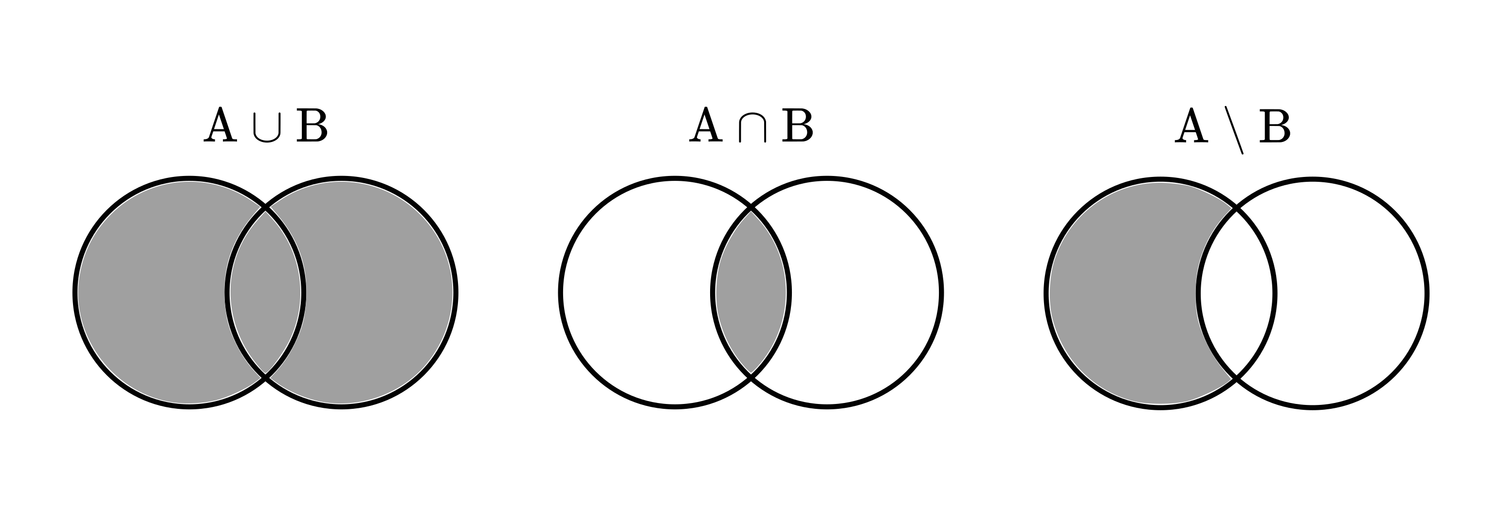
Fig. 3.1 Set operations visualized in Venn diagrams.
We can express set operations in plain English as well. For example, \( A \cup B \) means that “\( A \) or \( B \)“. Similarly, \( A \cap B \) means “\( A \) and \( B \)“, while \( A \setminus B \) is “\( A \) but not \( B \)“. When talking about probabilities, these will be useful for translating events to the language of set theory.
These set operations also have a lot of pleasant properties. For example, they behave nicely with respect to parentheses.
Theorem 3.1
Let \( A \), \( B \), and \( C \) be three sets. The union operation is
(a) associative, that is, \( A \cup (B \cup C) = (A \cup B) \cup C\),
(b) commutative, that is, \( A \cup B = B \cup A \).
Moreover, the intersection operation is also associative and commutative.
Finally,
(c) the union is distributive with respect to the intersection, that is, \( A \cup (B \cap C) = (A \cup B) \cap (A \cup C) \),
(d) and the intersection is distributive with respect to the union, that is, \( A \cap (B \cup C) = (A \cap B) \cup (A \cap C) \).
Union and intersection can be defined for an arbitrary number of operands. That is, if \( A_1, A_2, \dots, A_n \) are sets,
and similar for the intersection. Note that this is a recursive definition! Because of associativity, the order of parentheses doesn’t matter.
The associativity and commutativity might seem too abstract and trivial at the same time. However, this is not the case for all operations, so it is worth emphasizing to get used to the concepts. If you are curious, noncommutative operations are right under our noses. A simple example is string concatenation.
a = "string"
b = "concatenation"
a + b == b + a
False
3.2.2. De Morgan’s laws
One of the fundamental rules describes how set difference, union, and intersection behave together regarding set operations. These are called De Morgan’s laws.
Theorem 3.2 (De Morgan’s laws.)
Let \( A, B \), and \( C \) be three sets. Then
(a) \( A \setminus (B \cup C) = (A \setminus B) \cap (A \setminus C) \),
(b) \( A \setminus (B \cap C) = (A \setminus B) \cup (A \setminus C) \).
Proof. For simplicity, we are going to prove this using Venn diagrams. Although drawing a picture is not a “proper” mathematical proof, this is not a problem. We are here to understand things, not to get hung up on philosophy.
Here is the illustration.
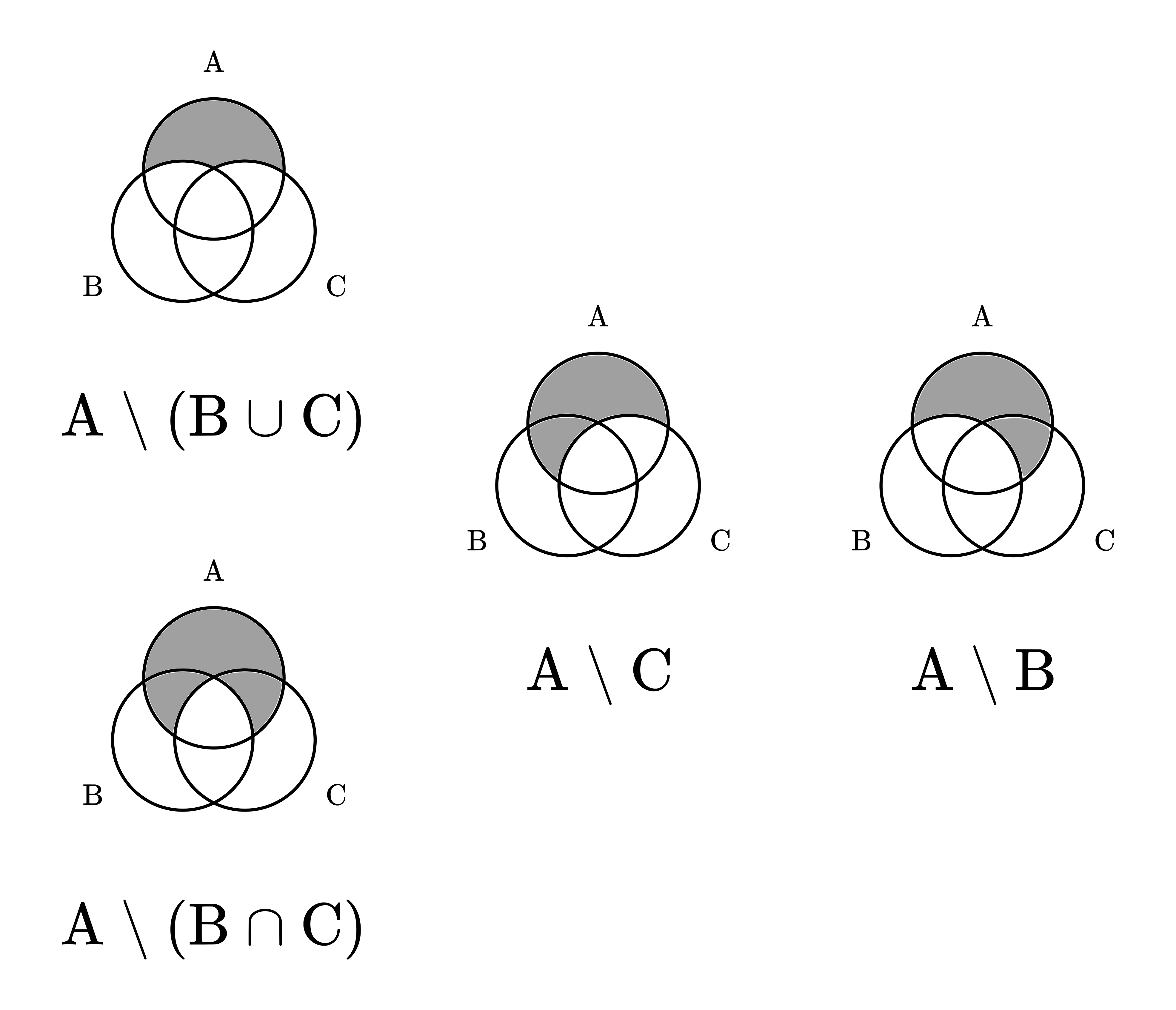
Fig. 3.2 De Morgan’s laws, illustrated on Venn diagrams.
Based on this, you can easily see both (a) and (b). \( \square \)
Note that De Morgan’s laws can be generalized to cover any number of sets. So, for any \( \Gamma \) index set,
3.3. The Cartesian product
One of the most fundamental ways to construct new sets is the Cartesian product.
Definition 3.2 (The Cartesian product.)
Let \( A \) and \( B \) be two sets. Their Cartesian product \( A \times B \) is defined by
The elements of the product are called tuples. Note that this operation is not associative nor commutative! To see this, consider that for example,
and
The Cartesian product for an arbitrary number of sets is defined with a recursive definition, just like we did with the union and intersection. So, if \( A_1, A_2, \dots, A_n \) are sets, then
Here, the elements are tuples of tuples of tuples of…, but to avoid writing an excessive number of parentheses, we can abbreviate it as \( (a_1, \dots, a_n) \). When the operands are the same, we usually write \( A^n \) instead of \( A \times \dots \times A \).
One of the most common examples is the Cartesian plane, which you probably have seen before.

To give you a machine learning-related example, let’s take a look at how we are usually given the data! Let’s focus on the famous Iris dataset, a subset of \( \mathbb{R}^4 \). Here, the axes represent sepal length, sepal width, petal length, and petal width.
Fig. 3.4 The sepal width, plotted against the sepal length in the Iris dataset. Source: scikit-learn documentation.
As the example demonstrates, Cartesian products are useful because they combine related information into a single mathematical structure. This is a recurring pattern in mathematics: building complex things from simpler building blocks and abstracting away the details by turning the result into yet another building block. (As one would do for creating complex software as well.)
3.4. The Russell paradox (optional)
Let’s return to a remark I made earlier: naively defining sets as collections of things is not going to cut it. In the following, we are going to see why. Prepare for some mind-twisting mathematics.
As we have seen, sets can be made of sets. For instance, \( \{ \mathbb{N}, \mathbb{Z}, \mathbb{R} \} \) is a collection of the most commonly used number sets. We might as well define the set of all sets, which we’ll denote with \( \Omega \).
With that, we can use the set-builder notation to describe the following collection of sets:
In plain English, \( S \) is a collection of sets that are not elements of themselves. Although this is weird, it looks valid. We used the property “\(A \notin A\)” to filter the set of all sets. What is the problem?
For one, we can’t decide if \( S \) is an element of \( S \) or not. If \( S \in S \), then by the defining property, \( S \notin S \). On the other hand, if \( S \notin S \), then by the definition, \( S \in S \). This is definitely very weird.
We can diagnose the issue by decomposing the set-builder notation. In general terms, it can be written as
where \( A \) is some set and \( T(x) \) is a property, that is, a true or false statement about \( x \). In the definition \( \{ A \in \Omega: A \notin A \} \), our abstract property is defined by
This is perfectly valid, so the problem must be in the other part: the set \( \Omega \). It turns out, the set of all sets is not a set. So, defining sets as a collection of things is not enough. Since sets are at the very foundations of mathematics, this discovery threw a giant monkey wrench into the machine around the late 19th - early 20th century, and it took lots of years and brilliant minds to fix it.
Fortunately, as machine learning practitioners, we don’t have to care about such low-level details as the axioms of set theory. For us, it is enough to know that a solid foundation exists somewhere. (Hopefully.)