Vectors in practice
Contents
2. Vectors in practice
So far, we have mostly talked about the theory of vectors and vector spaces. However, our ultimate goal is to build computational models for discovering and analyzing patterns in data. To put theory into practice, we will take a look at how vectors are represented in computations.
In computer science, there is a stark contrast between how we think about mathematical structures and how we represent them inside a computer. Until this point, our goal was to develop a mathematical framework that enables us to reason about the structure of data and its transformations effectively. We want a language that is
expressive,
easy to speak,
and as compact as possible.
However, our goals change when we aim to do computations instead of pure logical reasoning. We want implementations that are
easy to work with,
memory-efficient,
and fast to access, manipulate and transform.
These are often contradicting requirements, and particular situations might prefer one over the other. For instance, if we have plenty of memory but want to perform lots of computations, we can sacrifice size for speed. Because of all the potential use-cases, there are multiple formats to represent the same mathematical concepts. These are called data structures.
Different programming languages implement vectors differently. Because Python is ubiquitous in data science and machine learning, it’ll be our language of choice. In this chapter, we are going to study all the possible data structures in Python to see which one is suitable to represent vectors for high performance computations.
2.1. Tuples
In standard Python, two built-in data structures can be used to represent vectors: tuples and lists. Let’s start with tuples! They can be simply defined by enumerating their elements between two parentheses, separating them with commas.
v_tuple = (1, 3.5, -2.71, "a string", 42)
print(v_tuple)
(1, 3.5, -2.71, 'a string', 42)
type(v_tuple)
tuple
A single tuple can hold elements of various types. Even though we’ll exclusively deal with floats in computational linear algebra, this property is extremely useful for general purpose programming.
We can access the elements of a tuple by indexing. Just like in (almost) all other programming languages, indexing starts from zero. This is in contrast with mathematics, where we often start indexing from one. (Don’t tell this to anybody else, but it used to drive me crazy. I am a mathematician first.)
v_tuple[0]
1
The number of elements in a tuple can be accessed by calling the built-in
len function.
len(v_tuple)
5
Besides indexing, we can also access multiple elements by slicing.
v_tuple[1:4]
(3.5, -2.71, 'a string')
Slicing works by specifying the first and last elements with an optional step size, using the syntax
object[first:last:step].
Tuples are rather inflexible, as you cannot change their components. Attempting to do so results in a
TypeError, Python’s standard way of telling you that the object does not support the method you are trying to call (item
assignment).
v_tuple[0] = 2
---------------------------------------------------------------------------
TypeError                                 Traceback (most recent call last)
<ipython-input-8-5d8791fb815d> in <module>
----> 1 v_tuple[0] = 2

TypeError: 'tuple' object does not support item assignment
Besides that, extending the tuple with additional elements is also not supported. As we cannot change the state of a
tuple object in any way after it has been
instantiated, they are immutable. Depending on the use-case, immutability can be an advantage and a
disadvantage as well. Immutable objects eliminate accidental changes, but each operation requires the creation of a
new object, resulting in a computational overhead. Thus, tuples are not going to be optimal to represent large
amounts of data in complex computations.
This issue is solved by lists. Let’s take a look at them, and the new problems they introduce!
2.2. Lists
Lists are the workhorses of Python. In contrast with tuples, lists are extremely flexible and easy to use, albeit
this comes at the cost of runtime. Similarly to tuples, a
list object can be created by enumerating
its objects between square brackets, separated by commas.
v_list = [1, 3.5, -2.71, "qwerty"]
type(v_list)
list
Just like tuples, accessing the elements of a list is done by indexing or slicing.
We can do all kinds of operations on a list: overwrite its elements, append items, or even remove others.
v_list[0] = "this is a string"
v_list
['this is a string', 3.5, -2.71, 'qwerty']
This example illustrates that lists can hold elements of various types as well. Adding and removing elements can be
done with methods like append, push, pop, and remove.
Before trying that, let’s quickly take note of the memory address of our example list, which can be accessed by
calling the id function.
v_list_addr = id(v_list)
v_list_addr
140531937533320
This number simply refers to an address in my computer’s memory, where the
v_list object is located. Quite
literally, as this book is compiled on my personal computer.
Now, we are going to perform a few simple operations on our list and show that the memory address doesn’t change. Thus, no new object is created.
v_list.append([42])    # adding the list [42] to the end of our list
print(v_list)
['this is a string', 3.5, -2.71, 'qwerty', [42]]
id(v_list) == v_list_addr # adding elements doesn't create any new objects
True
v_list.pop(1)    # removing the element at the index "1"
print(v_list)
['this is a string', -2.71, 'qwerty', [42]]
id(v_list) == v_list_addr # removing elements still doesn't create any new objects
True
Unfortunately, adding lists together achieves a result that is completely different from our expectations.
[1, 2, 3] + [4, 5, 6]
[1, 2, 3, 4, 5, 6]
Instead of adding the corresponding elements together, like we want vectors to behave, the lists are concatenated. This feature is handy when writing general-purpose applications. However, this is not well-suited for scientific computations. “Scalar multiplication” also has strange results.
3*[1, 2, 3]
[1, 2, 3, 1, 2, 3, 1, 2, 3]
Multiplying a list with an integer repeats the list by the specified number of times. Given the behavior of the
+ operator on lists, this seems logical
as multiplication with an integer is repeated addition:
Overall, lists can do much more than we need to represent vectors. Although we potentially want to change elements of our vectors, we don’t need to add or remove elements from them, and we also don’t need to store objects other than floats. Can we sacrifice these extra features and obtain an implementation suitable for our purposes yet has a lightning-fast computational performance? Yes. Enter NumPy arrays.
2.3. NumPy arrays
Even though Python’s built-in data structures are amazing, they are optimized for ease of use, not for scientific computation. This problem was realized early on the language’s development and was addressed by the NumPy library.
One of the main selling points of Python is how fast and straightforward it is to write code, even for complex tasks. This comes at the price of speed. However, in machine learning, speed is crucial for us. When training a neural network, a small set of operations are repeated millions of times. Even a small percentage of improvement in performance can save hours, days, or even weeks in case of extremely large models.
Regarding speed, the C language is at the other end of the spectrum. C code is hard to write but executes blazing fast when done correctly. As Python is written in C, a tried and true method for achieving fast performance is to call functions written in C from Python. In a nutshell, this is what NumPy provides: C arrays and operations, all in Python.
To get a glimpse into the deep underlying issues with Python’s built-in data structures, we should put numbers and arrays under our magnifying glass. Inside a computer’s memory, objects are represented as fixed-length 0-1 sequences. Each component is called a bit. Bits are usually grouped into 8, 16, 32, 64, or even 128 sized chunks. Depending on what we want to represent, identical sequences can mean different things. For instance, the 8-bit sequence 00100110 can represent the integer 38 or the ASCII character “&”.
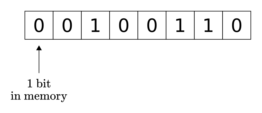
Fig. 2.1 An 8-bit object in memory.
By specifying the data type, we can decode binary objects. 32-bit integers are called
int32 types, 64-bit floats are
float64, and so on.
Since a single bit contains very little information, memory is addressed by dividing it into 32 or 64 bit sized chunks and numbering them consecutively. This address is a hexadecimal number, starting from 0. (For simplicity, let’s assume that the memory is addressed by 64 bits. This is customary in modern computers.)
A natural way to store a sequence of related objects (with matching data type) is to place them next to each other in the memory. This data structure is called an array.
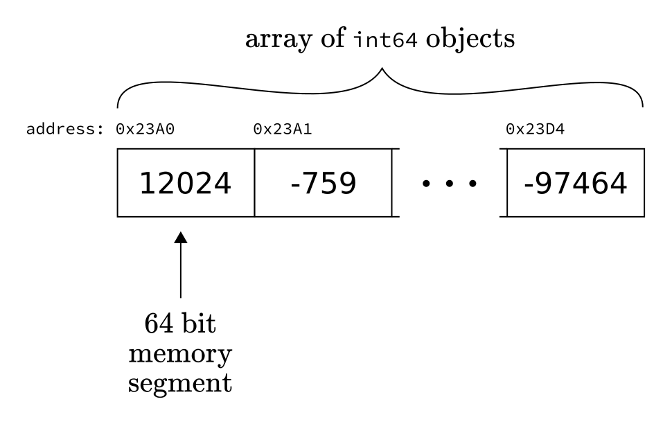
Fig. 2.2 An array of int64 objects.
By storing the memory address of the first object, say
0x23A0, we can instantly retrieve the k-th element by accessing the memory at
0x23A0 + k.
We call this the static array or often the C array because this is how it is done in the magnificent C language. Although this implementation of arrays is lightning fast, it is relatively inflexible. First, you can only store objects of a single type. Second, you have to know the size of your array in advance, as you cannot use memory addresses that overextend the pre-allocated part. Thus, before you start working with your array, you have to allocate memory for it. (That is, reserve space so that other programs won’t overwrite it.)
However, in Python, you can store arbitrarily large and different objects in the same list, with the option of removing and adding elements to it.
l = [2**142 + 1, "a string"]
l.append(lambda x: x)
l
[5575186299632655785383929568162090376495105,
 'a string',
 <function __main__.<lambda>(x)>]
In the example above, l[0] is an integer
so large that it doesn’t fit into 128 bits. Also, there are all kinds of objects in our list, including a function.
How is this possible?
Python’s list provides a flexible data
structure by
overallocating the memory and,
keeping memory addresses to the objects’ in the list instead of the objects themselves.
(At least in the most widespread CPython implementation.)
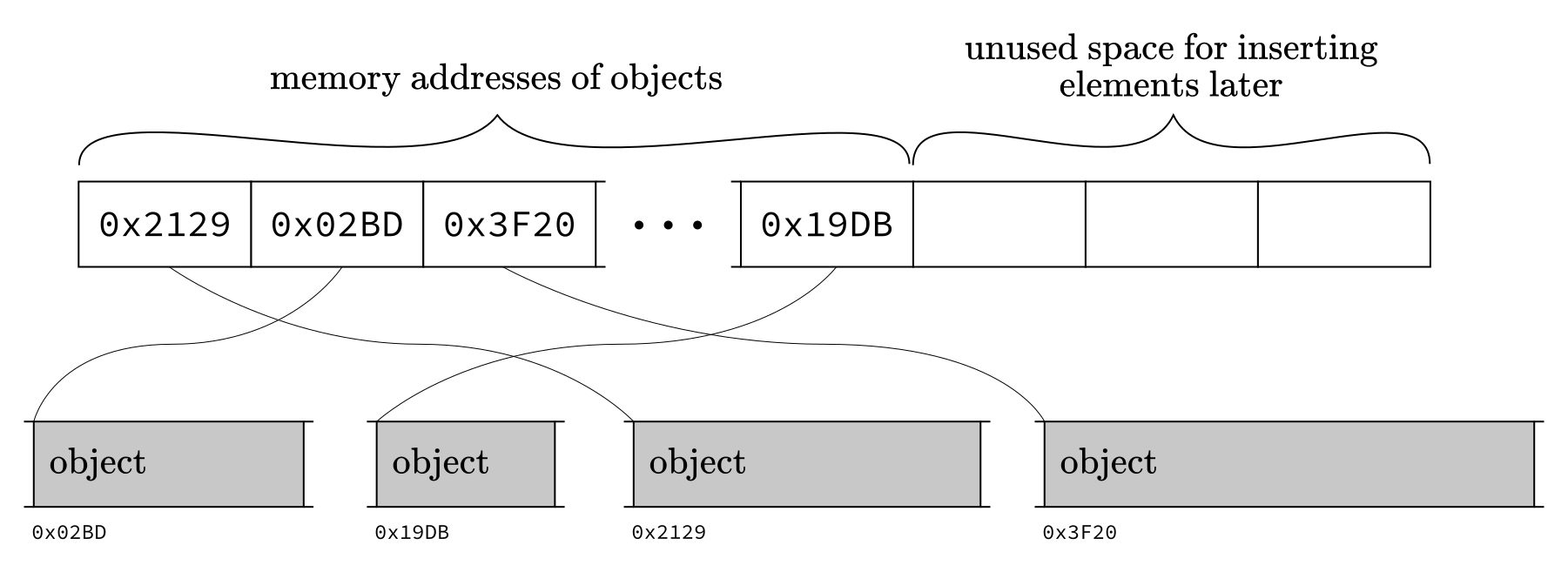
Fig. 2.3 CPython implementation of lists.
By checking the memory addresses of each object in our list
l, we can see that they are all over the memory.
[id(x) for x in l]
[140408800412080, 140408800519536, 140408800458816]
Due to the overallocation, deletion or insertion can always be done simply by shifting the remaining elements. Since the list stores the memory address of its elements, all types of objects can be stored within a single structure.
However, this comes at a cost. Because the objects are not contiguous in memory, we lose locality of reference, meaning that since we frequently access distant locations of the memory, our reads are much slower. Thus, looping over a Python list is not efficient, making it unsuitable for scientific computation.
So, NumPy arrays are essentially the good old C arrays in Python, with the user-friendly interface of Python lists. (If you have ever worked with C, you know how big of a blessing this is.) Let’s see how to work with them!
First, we import the numpy library. (To
save on the characters, it is customary to import it as
np.)
import numpy as np
The main data structure is the np.ndarray, short for n-dimensional array. We can use the
np.array function to create NumPy arrays
from standard Python containers or initialized from scratch. (Yes, I know. This is confusing, but you’ll get used to
it. Just take a mental note that
np.ndarray is the class, and
np.array is the function you use to
create NumPy arrays from Python objects.)
X = np.array([87.7, 4.5, -4.1, 42.1414, -3.14, 2.001]) # creating a NumPy array from a Python list
X
array([87.7 , 4.5 , -4.1 , 42.1414, -3.14 , 2.001 ])
np.ones(shape=7) # initializing a NumPy array from scratch using ones
array([1., 1., 1., 1., 1., 1., 1.])
np.zeros(shape=5) # initializing a NumPy array from scratch using zeros
array([0., 0., 0., 0., 0.])
We can even initialize NumPy arrays using random numbers. Later, when talking about probability theory, we’ll discuss this functionality in detail, as the library covers a wide range of probability distributions.
np.random.rand(10)
array([0.66339028, 0.19520763, 0.60535065, 0.52306207, 0.24778104,
       0.99992155, 0.76469949, 0.61753093, 0.46085152, 0.22215355])
Most importantly, when we have a given array, we can initialize another one with the same dimensions using the
np.zeros_like, np.ones_like, and np.empty_like functions.
np.zeros_like(X)
array([0., 0., 0., 0., 0., 0.])
Just like Python lists, NumPy arrays support item assignments and slicing.
X[0] = 1545.215
X
array([1545.215 , 4.5 , -4.1 , 42.1414, -3.14 , 2.001 ])
X[1:4]
array([ 4.5 , -4.1 , 42.1414])
However, as expected, you can only store a single data type within each
ndarray. When trying to assign a string as the first element, we get an error message.
X[0] = "str"
---------------------------------------------------------------------------
ValueError                                Traceback (most recent call last)
<ipython-input-34-d996c0d86300> in <module>
----> 1 X[0] = "str"

ValueError: could not convert string to float: 'str'
As you might have guessed, every
ndarray has a data type attribute that
can be accessed at ndarray.dtype. If a conversion can be made between the value to be assigned and the data type, it is automatically performed,
making the item assignment successful.
X.dtype
dtype('float64')
val = 23
type(val)
int
X[0] = val
X
array([23. , 4.5 , -4.1 , 42.1414, -3.14 , 2.001 ])
NumPy arrays are iterable, just like other container types in Python.
for x in X:
    print(x)
23.0
4.5
-4.1
42.1414
-3.14
2.001
Are these suitable to represent vectors? Yes. Let’s see why!
2.3.1. NumPy arrays as vectors
Let’s talk about vectors once more. From now on, we are going to use NumPy
ndarray-s to model vectors.
v_1 = np.array([-4.0, 1.0, 2.3])
v_2 = np.array([-8.3, -9.6, -7.7])
The addition and scalar multiplication operations are supported by default and perform as expected.
v_1 + v_2 # adding v_1 and v_2 together as vectors
array([-12.3, -8.6, -5.4])
10.0*v_1 # multiplying v_1 with a scalar
array([-40., 10., 23.])
v_1 * v_2 # the elementwise product of v_1 and v_2
array([ 33.2 , -9.6 , -17.71])
np.zeros(shape=3) + 1
array([1., 1., 1.])
Because of the dynamic typing of Python, we can (often) plug in NumPy arrays into functions intended for scalars.
def f(x):
    return 3*x**2 - x**4
f(v_1)
array([-208. , 2. , -12.1141])
So far, NumPy arrays satisfy almost everything we require to represent vectors. There is only one box to be
ticked: performance. To investigate this, we measure the execution time with Python’s built-in
timeit tool.
In its first argument, timeit takes a function to be executed and timed. Instead of passing a function object, it also accepts executable statements as a string. Since function calls have a significant computational overhead in Python, we are passing code rather than a function object in order to be precise with the time measurements.
Below, we compare adding together two NumPy arrays vs. Python lists containing a thousand zeros.
from timeit import timeit


n_runs = 100000
size = 1000


t_add_builtin = timeit(
    "[x + y for x, y in zip(v_1, v_2)]",
    setup=f"size={size}; v_1 = [0 for _ in range(size)]; v_2 = [0 for _ in range(size)]",
    number=n_runs
)

t_add_numpy = timeit(
    "v_1 + v_2",
    setup=f"import numpy as np; size={size}; v_1 = np.zeros(shape=size); v_2 = np.zeros(shape=size)",
    number=n_runs
)


print(f"Built-in addition:       \t{t_add_builtin} s")
print(f"NumPy addition:          \t{t_add_numpy} s")
print(f"Performance improvement: \t{100*t_add_builtin/t_add_numpy}% speedup")
Built-in addition:       	3.3502430509997794 s
NumPy addition:          	0.06488390699996671 s
Performance improvement: 	5163.4422245896785% speedup
NumPy arrays are much-much faster. This is because they are
contiguous in memory,
homogeneous in type,
with operations implemented in C.
This is just the tip of the iceberg. We have only seen a small part of it, but NumPy provides much more than a fast data structure. As we progress in the book, we’ll slowly dig deeper and deeper, eventually discovering the vast array of functionalities it provides.
2.3.2. Why NumPy instead of TensorFlow or PyTorch?
If you are already familiar with some deep learning frameworks, you might ask: why are we studying NumPy instead of them? The answer is simple: because all state-of-the-art libraries are built on its legacy. Modern tensor libraries are essentially clones of NumPy, with GPU support. Thus, most NumPy knowledge translates directly to TensorFlow and PyTorch. If you understand how it works on a fundamental level, you’ll have a headstart in more advanced frameworks.
Moreover, our goal is to implement our neural network from scratch by the end of the book. To understand every nook and cranny, we don’t want to use built-in algorithms like backpropagation. We’ll create our own!
2.4. Is NumPy really faster than Python?
NumPy is designed to be faster than vanilla Python. Is this really the case? Not all the time. If you use it wrong, it might even hurt performance! To know when it is beneficial to use NumPy, we will look at why exactly it is faster in practice.
To simplify the investigation, our toy problem will be random number generation. Suppose that we need just a single random number. Should we use NumPy? Let’s test it! We are going to compare it with the built-in random number generator by running both ten million times, measuring the execution time.
from numpy.random import random as random_np
from random import random as random_py


n_runs = 10000000
t_builtin = timeit(random_py, number=n_runs)
t_numpy = timeit(random_np, number=n_runs)

print(f"Built-in random:\t{t_builtin} s")
print(f"NumPy random:   \t{t_numpy} s")
Built-in random:	0.2327952079995157 s
NumPy random:   	1.9404740369991487 s
For generating a single random number, NumPy is significantly slower. Why is this the case? What if we need an array instead of a single number? Will this also be slower?
This time, let’s generate a list/array of a thousand elements.
size = 1000
n_runs = 10000

t_builtin_list = timeit(
    "[random_py() for _ in range(size)]",
    setup=f"from random import random as random_py; size={size}",
    number=n_runs
)

t_numpy_array = timeit(
    "random_np(size)",
    setup=f"from numpy.random import random as random_np; size={size}",
    number=n_runs
)

print(f"Built-in random with lists:\t{t_builtin_list}s")
print(f"NumPy random with arrays:  \t{t_numpy_array}s")
Built-in random with lists:	0.4184184540008573s
NumPy random with arrays:  	0.062079527000605594s
(Again, I don’t want to wrap the timed expressions in lambdas since function calls have an overhead in Python. I
want to be as precise as possible, so I pass them as strings to the
timeit function.)
Things are looking much different now. When generating an array of random numbers, NumPy wins hands down.
There are some curious things about this result as well. First, we generated a single random number 10 000 000 times. Second, we generated an array of 1000 random numbers 10 000 times. In both cases, we have 10 000 000 random numbers in the end. Using the built-in method, it took ~2x time when we put them in a list. However, with NumPy, we see a ~30x speedup compared to itself when working with arrays!
2.4.1. Dissecting the code: profiling with cProfiler
To see what happens behind the scenes, we are going to profile the code using cProfiler. With this, we’ll see exactly how many times a given function was called and how much time we spent inside them.
(To make profiling work from Jupyter Notebooks, we need to do some Python magic first. Feel free to disregard the contents of the next cell; this is just to make sure that the output of the profiling is printed inside the notebook.)
from IPython.core import page
page.page = print
Let’s take a look at the built-in function first. In the following function, we create 10 000 000 random numbers, just as before.
def builtin_random_single(n_runs):
    for _ in range(n_runs):
        random_py()
From Jupyter Notebooks, where this book is written, cProfiler can be called with the magic command
%prun.
n_runs = 10000000

%prun builtin_random_single(n_runs)
         10000004 function calls in 1.037 seconds

   Ordered by: internal time

   ncalls  tottime  percall  cumtime  percall filename:lineno(function)
        1    0.630    0.630    1.037    1.037 <ipython-input-45-73f06baff02e>:1(builtin_random_single)
 10000000    0.407    0.000    0.407    0.000 {method 'random' of '_random.Random' objects}
        1    0.000    0.000    1.037    1.037 {built-in method builtins.exec}
        1    0.000    0.000    1.037    1.037 <string>:1(<module>)
        1    0.000    0.000    0.000    0.000 {method 'disable' of '_lsprof.Profiler' objects}
There are two important columns here for our purposes.
ncalls shows how many times a function
was called, while tottime is the total
time spent in a function, excluding time spent in subfunctions.
The built-in function
random.random() was called 10 000 000
times as expected, and the total time spent in that function was 0.407 seconds. (If you are running this notebook
locally, this number is going to be different.)
What about the NumPy version? The results are surprising.
def numpy_random_single(n_runs):
    for _ in range(n_runs):
        random_np()
%prun numpy_random_single(n_runs)
         10000004 function calls in 2.820 seconds

   Ordered by: internal time

   ncalls  tottime  percall  cumtime  percall filename:lineno(function)
 10000000    2.174    0.000    2.174    0.000 {method 'random' of 'numpy.random.mtrand.RandomState' objects}
        1    0.646    0.646    2.820    2.820 <ipython-input-47-db45b38db7dd>:1(numpy_random_single)
        1    0.000    0.000    2.820    2.820 {built-in method builtins.exec}
        1    0.000    0.000    2.820    2.820 <string>:1(<module>)
        1    0.000    0.000    0.000    0.000 {method 'disable' of '_lsprof.Profiler' objects}
Similarly as before, the
numpy.random.random() function was
indeed called 10 000 000 times as expected. Yet, the script spent significantly more time in this function than in
the Python built-in random before. Thus, it is more costly per call.
When we start working with large arrays and lists, things change dramatically. Next, we generate a list/array of 1000 random numbers, while measuring the execution time.
def builtin_random_list(size, n_runs):
    for _ in range(n_runs):
        [random_py() for _ in range(size)]
size = 1000
n_runs = 10000

%prun builtin_random_list(size, n_runs)
         10010004 function calls in 1.138 seconds

   Ordered by: internal time

   ncalls  tottime  percall  cumtime  percall filename:lineno(function)
    10000    0.641    0.000    1.089    0.000 <ipython-input-49-d0bf27f76fac>:3(<listcomp>)
 10000000    0.448    0.000    0.448    0.000 {method 'random' of '_random.Random' objects}
        1    0.049    0.049    1.138    1.138 <ipython-input-49-d0bf27f76fac>:1(builtin_random_list)
        1    0.000    0.000    1.138    1.138 {built-in method builtins.exec}
        1    0.000    0.000    1.138    1.138 <string>:1(<module>)
        1    0.000    0.000    0.000    0.000 {method 'disable' of '_lsprof.Profiler' objects}
As we see, about 60% of the time was spent on the list comprehensions: 10 000 calls, 0.641s total. (Note that
tottime doesn’t count subfunction calls
like calls to random.random() here.)
Now we are ready to see why NumPy is faster when used right.
def numpy_random_array(size, n_runs):
    for _ in range(n_runs):
        random_np(size)
%prun numpy_random_array(size, n_runs)
         10004 function calls in 0.066 seconds

   Ordered by: internal time

   ncalls  tottime  percall  cumtime  percall filename:lineno(function)
    10000    0.064    0.000    0.064    0.000 {method 'random' of 'numpy.random.mtrand.RandomState' objects}
        1    0.001    0.001    0.066    0.066 <ipython-input-51-219ecab2e001>:1(numpy_random_array)
        1    0.000    0.000    0.066    0.066 {built-in method builtins.exec}
        1    0.000    0.000    0.066    0.066 <string>:1(<module>)
        1    0.000    0.000    0.000    0.000 {method 'disable' of '_lsprof.Profiler' objects}
With each of the 10 000 function calls, we get a
numpy.ndarray of 1000 random numbers.
The reason why NumPy is fast when used right is that its arrays are extremely efficient to work with. They are
like C arrays instead of Python lists. As we have seen, there are two significant differences between them.
-
Python lists are dynamic, so for instance, you can append and remove elements. NumPy arrays have fixed lengths, so you cannot add or delete without creating a new one.
Python lists can hold several data types simultaneously, while a NumPy array can only contain one.
So, NumPy arrays are less flexible but significantly more performant. When this additional flexibility is not needed, NumPy outperforms Python.
2.4.2. Where is the break-even point?
To see precisely at which size does NumPy overtakes Python in random number generation, we can compare the two by measuring the execution times for several sizes.
sizes = list(range(1, 100))

runtime_builtin = [
    timeit(
        "[random_py() for _ in range(size)]",
        setup=f"from random import random as random_py; size={size}",
        number=100000
    )
    for size in sizes
]


runtime_numpy = [
    timeit(
        "random_np(size)",
        setup=f"from numpy.random import random as random_np; size={size}",
        number=100000
    )
    for size in sizes
]
import matplotlib.pyplot as plt


with plt.style.context("seaborn-white"):
    plt.figure(figsize=(10, 5))
    plt.plot(sizes, runtime_builtin, label="built-in")
    plt.plot(sizes, runtime_numpy, label="NumPy")
    plt.xlabel("array size")
    plt.ylabel("time (seconds)")
    plt.title("Runtime of random array generation")
    plt.legend()
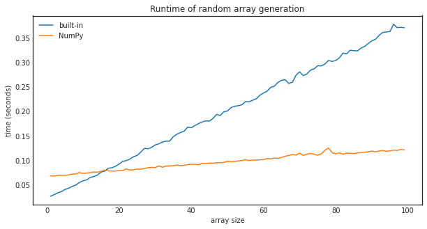
Around 20, NumPy starts to beat Python in performance. Of course, this number might be different for other operations like calculating the sine or adding numbers together, but the tendency will be the same. Python will slightly outperform NumPy for small input sizes, but NumPy wins by a large margin as the size grows.